We often have intuitions about the probability distribution of a variable that we would like to translate into a formal specification of a distribution. Transforming our beliefs into a fully specified probability distribution allows us to further manipulate the distribution in useful ways.

For example, you believe that the cost of a medication is a positive number that’s about 10, but with a long right tail: say, a 10% probability of being more than 100. To use this cost estimate in a Monte Carlo simulation, you need to know exactly what distribution to plug in. Or perhaps you have a prior about the effect of creatine on cognitive performance, and you want to formally update that prior using Bayes’ rule when a new study comes out. Or you want to make a forecast about a candidate’s share of the vote and evaluate the accuracy of your forecast using a scoring rule.

In most software, you have to specify a distribution by its parameters, but these parameters are rarely intuitive. The normal distribution’s mean and standard deviation are somewhat intuitive, but this is the exception rather than the rule. The lognormal’s mu and sigma correspond to the mean and standard deviation of the variable’s logarithm, something I personally have no intuitions about. And I don’t expect good results if you ask someone to supply a beta distribution’s alpha and beta shape parameters.

I have built a tool that creates a probability distribution (of a given family) from user-supplied quantiles, sometimes also called percentiles. Quantiles are points on the cumulative distribution function: $(p,x)$ pairs such that $P(X<x)=p$. To illustrate what quantiles are, we can look at the example distribution below, which has a 50th percentile (or median) of -1 and a 90th percentile of 10.

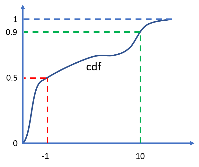
A cumulative distribution function with a median of -1 and a 90th percentile of 10

The code is on GitHub, and the webapp is here.

Let’s run through some examples of how you can use this tool. At the end, I will discuss how it compares to other probability elicitation software, and why I think it’s a valuable addition.

Traditional distributions

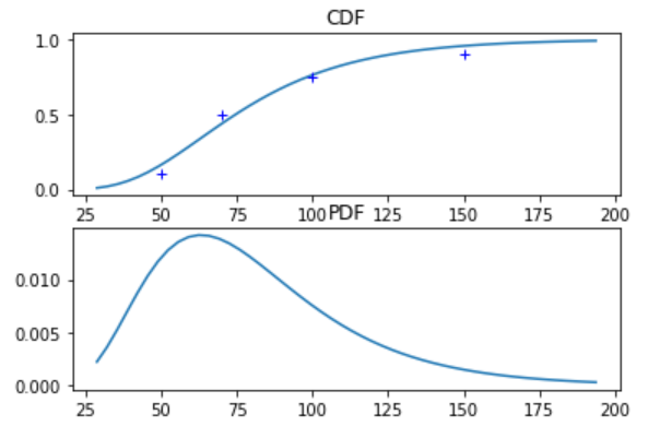
The tool supports the normal and lognormal distributions, and more of the usual distribution families could easily be added. The user supplies the distribution family, along with an arbitrary number of quantiles. If more quantiles are provided than the distribution has parameters (more than two in this case), the system is over-determined. The tool then uses least squares to find the best fit.

This is some example input:

family = 'lognormal'
quantiles = [(0.1,50),(0.5,70),(0.75,100),(0.9,150)]

And the corresponding output:

More than two quantiles provided, using least squares fit

Lognormal distribution
mu 4.313122980928514
sigma 0.409687416531683

quantiles:
0.01 28.79055927521217
0.1 44.17183774344628
0.25 56.64439363937313
0.5 74.67332855521319
0.75 98.44056294458953
0.9 126.2366766332274
0.99 193.67827989071688

Metalog distribution

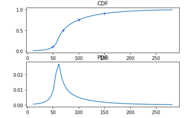
The feature I am most excited about, however, is the support for a new type of distribution developed specifically for the purposes of flexible elicitation from quantiles, called the meta-logistic distribution. It was first described in Keelin 2016, which puts it at the cutting edge compared to the venerable normal distribution invented by Gauss and Laplace around 1810. The meta-logistic, or metalog for short, does not use traditional parameters. Instead, it can take on as many terms as the user provides quantiles, and adopts whatever shape is needed to fit these quantiles very closely. Closed-form expressions exist for its quantile function (the inverse of the CDF) and for its PDF. This leads to attractive computational properties (see footnote)¹.

Keelin explains that

[t]he metalog distributions provide a convenient way to translate CDF data into smooth, continuous, closed-from distribution functions that can be used for real-time feedback to experts about the implications of their probability assessments.

The metalog quantile function is derived by modifying the logistic quantile function,

by letting $\mu$ and $s$ depend on $y$ instead of being constant.

As Keelin writes, given a systematically increasing $s$ as one moves from left to right, a right skewed distribution would result. And a systematically decreasing $\mu$ as one moves from left to right would make the distribution spikier in the middle with correspondingly heavier tails.

By modifying $s$ and $\mu$ in ever more complex ways we can make the metalog take on almost any shape. In particular, in most cases the metalog CDF passes through all the provided quantiles exactly². Moreover, we can specify the metalog to be unbounded, to have arbitrary bounds, or to be semi-bounded above or below.

Instead of thinking about which of several highly constraining distribution families to use, just choose the metalog and let your quantiles speak for themselves. As Keelin says:

one needs a distribution that has flexibility far beyond that of traditional distributions – one that enables “the data to speak for itself” in contrast to imposing unexamined and possibly inappropriate shape constraints on that data.

For example, we can fit an unbounded metalog to the same quantiles as above:

family = 'metalog'
quantiles = [(0.1,50),(0.5,70),(0.75,100),(0.9,150)]
metalog_leftbound = None
metalog_rightbound = None

Meta-logistic distribution

quantiles:
0.01 11.968367580205552
0.1 50.000000000008185
0.25 58.750000000005215
0.5 70.0
0.75 100.00000000000519
0.9 150.00000000002515
0.99 281.7443263650518

The metalog’s actual parameters (as opposed to the user-supplied quantiles) have no simple interpretation and are of no use unless the next piece of software you’re going to use knows what a metalog is. Therefore the program doesn’t return the parameters. Instead, if we want to manipulate this distribution, we can use the expressions of the PDF and CDF that the software provides, or alternatively export a large number of samples into another tool that accepts distributions described by a list of samples (such as the Monte Carlo simulation tool Guesstimate). By default, 5000 samples will be printed; you can copy and paste them.

Approaches to elicitation

How does this tool compare to other approaches for creating subjective belief distributions? Here are the strategies I’ve seen.

Belief intervals

The first approach is to provide a belief interval that is mapped to some fixed quantiles, e.g. a 90% belief interval (between the 0.05 and 0.95 quantile) like on Guesstimate. Metaculus provides a graphical way to input the same data, allowing the user to drag the quantiles across a line under a graph of the PDF. This is the simplest and most user-friendly approach. The tool I built incorporates the belief interval approach while going beyond it in two ways. First, you can provide completely arbitrary quantiles, instead of specifically the 0.05 and 0.95 – or some other belief interval symmetric around 0.5. Second, you can provide more than two quantiles, which allows the user to query intuitive information about more parts of the distribution.

Guesstimate

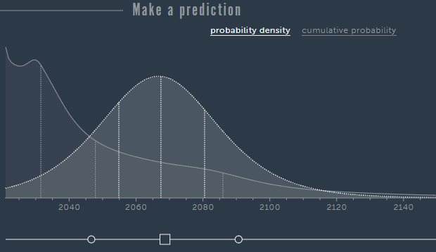
Metaculus

Drawing

Another option is to draw the PDF on a canvas, in free form, using your mouse. This is the very innovative approach of probability.dev.³

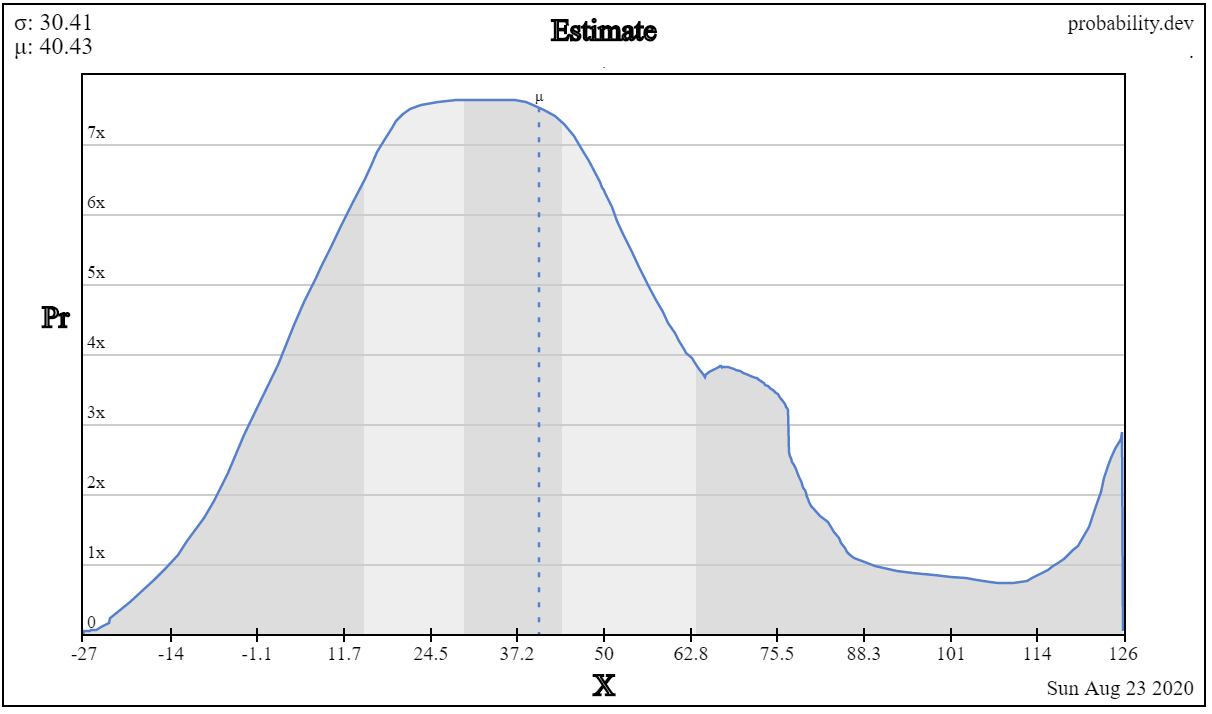
probability.dev

Ought’s elicit

Ought’s elicit lets you provide quantiles like my tool, or equivalently bins with some probability mass in each bin⁴. The resulting distribution is by default piecewise uniform (the cdf is piecewise linear), but it’s possible to apply smoothing. It has all the features I want, the drawback is that it only supports bounded distributions⁵.

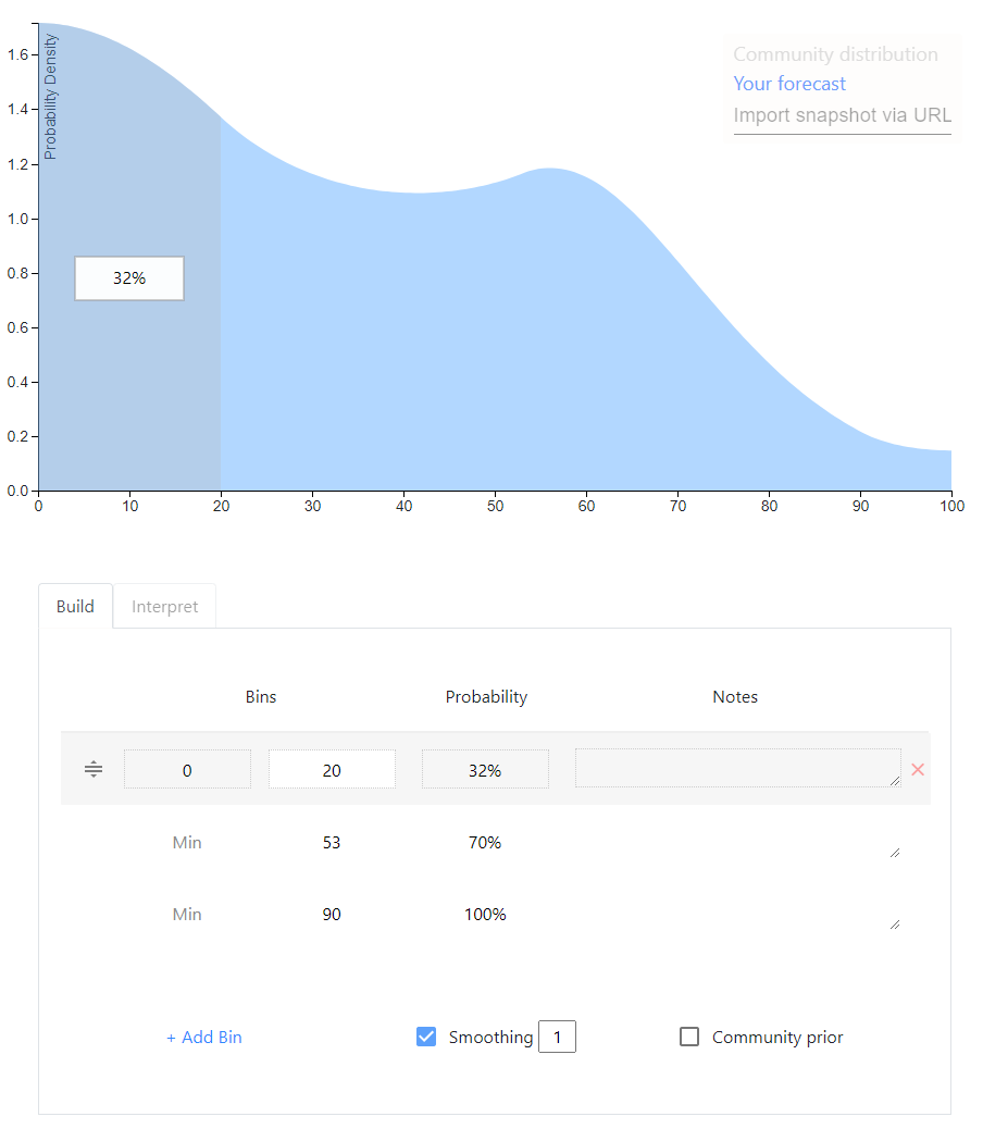
Elicit

Mixtures

A meta-level approach that can be applied to any of the above is to allow the user to specify a mixture distribution, a weighted average of distributions. For example, 1/3 weight on a normal(5,5) and 2/3 weight on a lognormal(1,0.75). My opinion on mixtures is that they are good if the user is thinking about the event disjunctively; for example, she may be envisioning two possible scenarios, each of which she has a distribution in mind for. But on Metaculus and Foretold my impression is that mixtures are often used to indirectly achieve a single distribution whose rough shape the user had in mind originally.

The future

This is an exciting space with many recent developments. Guesstimate, Metaculus, Elicit and the metalog distribution have all been created in the last 5 years.